Getting started
Tutorial
Getting started
In this tutorial we are processing PAR-CLIP data of the Nrd1 protein in S. cerevisiae. For more information on the biological role of Nrd1 and the PAR-CLIP experiment, please refer to [SSK+13].
Please follow this link and download mockinbird_tutorial_nomock.tar.gz which contains all data required for completing this tutorial.
Running the preprocessing
Having installed and loaded the mockinbird enviroment according to the installation guide, use cd to navigate into the tutorial directory from the shell. First we run the preprocessing pipeline to obtain predicted binding sites at single nucleotide resolution:
mockinbird preprocess nrd1.fastq nrd1 nrd1 preprocess.yaml
Running the full pipeline will take some time. The current status will be logged to the shell.
Inspecting the results
Once the pipeline finished successfully, it is time to inspect the results.
Checking reads and mapping
The number of generated files may be daunting at first. Following route can be used to obtain a first impression of the data.
First have a look at the mapping output, which is printed to stdout and
can also be found in preprocess.log
# reads processed: 20442544
# reads with at least one reported alignment: 1273512 (6.23%)
# reads that failed to align: 17229731 (84.28%)
# reads with alignments suppressed due to -m: 1939301 (9.49%)
Reported 1273512 alignments to 1 output stream(s)
A sufficient number of mapped reads is crucial for predicting high confidence binding sites.
Now check transition_frequencies_nuc_mutations.pdf and verify that
the characteristic PAR-CLIP mutation (T->C for 4sU) is the dominant transition:
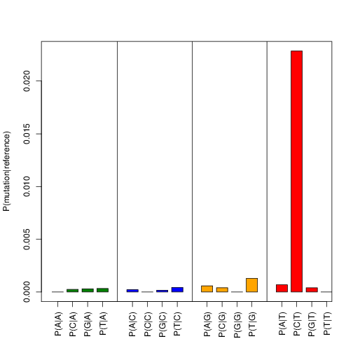
Fig. 1 Transition frequencies
The FastQC reports in fastQC_raw and fastQC_clipped can be consulted to obtain
a general overview over the quality of the sequencing library. It is adviced to pay special attention to the
read quality and the overrepresented sequences.
A quick glance at clipped_len_distr.pdf will give an overview over the size
distribution of the RNA inserts. The optimal size distribution depends on the the genome size.
For yeast we will only map reads of size 20 nt and longer. Here, more than 80% of the clipped reads are eligible for mapping.
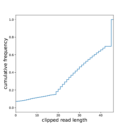
Fig. 2 Insert size distribution
Checking transition profiles
BamPPModule creates a bam_analysis folder with several diagnostic plots that
give a more detailed overview over the transition properties in reads.
BamPPModule also allows to manipulate and filter aligned reads.
All diagnostic plots are created twice. The plots before filtering can be found in the subfolder
pre_fil_data.
Plots after filtering are stored in post_fil_data.
First browse through the transition profiles after filtering. The PAR-CLIP specific mutation should dominate all other transitions and be roughly uniformly distributed over all positions. Spikes at specific positions hint towards mismapping and/or abundance of PCR duplicates. The ratio of specific to unspecific mutations will drop towards the ends of the reads due to (adapter) contamination. You may want to drop mutations at the edges. Please refer to the documentation of BamPPModule for how this can be done.
Transition profiles will degenerate for shorter read lengths. Increasing the minimum length of accepted alignments will therefore increase the signal to noise ratio.
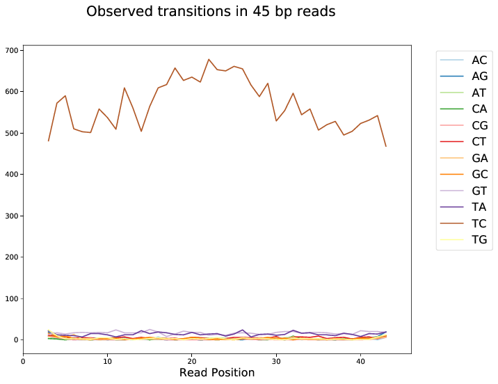
Fig. 3 Transition profile for alignments of length 45 bp
Additional aspects
The bam_analysis folder contains several other plots that help chosing suitable pipeline
configuration options:
mismatch_profiles: the total mutation frequency profiles per positionlength_transition_plot.pdf: the PAR-CLIP specific mutation frequency for different alignment sizesquality_transition_plot.pdf: the PAR-CLIP specific mutation frequency for different quality scoresmapped_lengths.pdf: the length frequencies of aligned reads
The configuration file
The pipeline configuration of the preprocessing run can be found in preprocess.yaml.
In the following the preprocessing file for the tutorial is explained in more depth:
{% set data_dir = "data" %}

{% set genome_fasta = data_dir + "/genome.fa" %}
{% set mock_pileup = data_dir + "/mock.mpileup" %}
{% set mock_statistics = data_dir + "/mock_stat.json" %}
{% set norm_pileup = data_dir + "/normalization.mpileup" %}
{% set bowtie_index = data_dir + "/bowtie_index/genome" %}

# setting mock_processing to True will only process the mock. Setting to `False` will run the full
# pipeline
{% set mock_processing = False %}
The first block uses jinja syntax to define a set of
variables. Path can be defined absolutely, or relative to the directory that contains the config file preprocess.yaml.
general:
    adapter5prime: GTTCAGAGTTCTACAGTCCGACGATC
    adapter3prime: TGGAATTCTCGGGTGCCAAGG
    genomefasta: {{ genome_fasta }}
    normalization_pileup: {{ norm_pileup }}
    rmTemp: yes
    n_threads: 4

reads:
    bc_5prime: 5
    bc_3prime: 0
    min_len: 20
    reference_nucleotide: T
    mutation_nucleotide: C
The second block defines general and read-specific configuration. Here you can define the minimum read length, presence and size of UMIs, sequencing adapter sequences and more.For a detailed description of all available settings please refer to the section on Preprocessing configuration.
The next parts define the preprocessing pipeline as a list of modules.
pipeline:
    - FastQCModule:
        outdir_name: fastQC_raw

    - UmiToolsExtractModule

    - SkewerAdapterClippingModule

    - ClippyAdapterClippingModule:
        clipped_5prime_bc: True

    - FastQCModule:
        outdir_name: fastQC_clipped
The tutorial pipeline performs following steps before mapping:
- a report of the quality of the raw reads is generated using
FastQCumi_toolsremoves the five random nucleotides from the 5’ end of the readsskewerclips the 3’ sequencing adapterclippyclips 5’ adapters and drops adapter dimers- finally a second
FastQCreport is generated to check the clipping results
- BowtieMapModule:
    genome_index: {{ bowtie_index }}

- BamPPModule:
    remove_n_edge_mut: 2
    max_mut_per_read: 1
    min_mismatch_quality: 20

- SortIndexModule:
   keep_all: yes

- UmiToolsDedupModule

- SortIndexModule:
   keep_all: yes

- PileupModule:
   keep_all: yes

- BamStatisticsModule
The second set of modules
- maps the clipped reads with
bowtie - postprocesses the obtained alignments and plots transitions statistics
- removes PCR duplicates
- calculates an
mpileupfile - calculates bam statistics
If mock_processing is set to True, the pipeline ends here, as the mpileup file and the
bam statistics of the mock are required for the prediction modules.
When processing a factor of interest, the following modules run the mock-based prediction:
{% if not mock_processing %}

    - PredictionSitesModule:
        sites_file: {{ data_dir }}/genome.sites
        fasta_file: {{ genome_fasta }}
        transition_nucleotide: T

    - MockTableModule:
        mock_table: {{ data_dir }}/mock.table
        mock_pileup: {{ mock_pileup }}

    - TransitionTableModule

    - LearnMockModule:
        mock_model: mock_model/model.pkl
        mock_statistics: {{ mock_statistics }}
        n_mixture_components: 5
        em_iterations: 250

    - MockinbirdModule

    - NormalizationModule
    - QuantileCapModule
{% endif %}
The last steps calculate an occupancy by dividing the number of transitions by
the coverage of an RNAseq experiment conducted under PAR-CLIP conditions and cap the occupancy
values at the 0.95 quantile.
The final output is a .table file. We will create plots from it in section Running the postprocessing.
Running the postprocessing
The postprocessing can be started from the tutorial directory by
mockinbird postprocess nrd1 nrd1_pp postprocess.yaml
in a standard installation, or
docker run -v $PWD:/data soedinglab/mockinbird postprocess nrd1 nrd1_pp postprocess.yaml
in case you are using the docker container.
The output of the preprocessing phase is a PAR-CLIP table file, here nrd1_capped.table.
Each line lists one predicted PAR-CLIP binding site, along with the number of PAR-CLIP transitions,
the read coverage, a confidence and an occupancy score and the estimated posterior probability:
seqid   position        transitions     coverage        score   strand  occupancy       posterior
chrI    32601   4       4       6.352710158543762       -       0.15384615384615385     0.772109761967
chrI    35562   4       5       5.292152965717071       +       0.0223463687150838      0.539841709238
chrI    35805   5       5       9.376254703871467       +       0.03184713375796178     0.98585024515
The postprocessing pipeline allows to do general purpose downstream analyses:
Meta-gene plot
Meta gene plots visualize the PAR-CLIP signal over the body of aligned annotations (meta-genes).
_centerplot_bs creates a metagene plot that is aligned at the start and end of the annotation.

Fig. 4 Meta-gene plot of the PAR-CLIP occupancies.
In this example we align TIF-seq gene annotation [PWS13]. 95% confidence intervals calculated by bootstrap sampling the annotations are shaded.
The configuration file
postprocess.yaml contains the configuration of the postprocessing pipeline used for the tutorial.
In the beginning several jinja variables are defined for later use.
{% set data_dir = "data" %}

{% set gff_db = data_dir + "/Annotations" %}
{% set genome_file = data_dir + "/genome.fa" %}
{% set full_annotation = gff_db + "/R64-2-1_genes.gff" %}
{% set filter_gff = full_annotation %}
{% set negative_set_gff = full_annotation %}
{% set intron_gff = gff_db + "/R64-2-1_introns.gff" %}

{% set bootstrap_iter = 1000 %}
{% set n_processes = 6 %}
The first module removes PAR-CLIP sites falling into tRNA, snRNA, snoRNA and rRNA from the table file.
pipeline:

    - GffFilterModule:
        filter_gff: {{ filter_gff }}
        padding_bp: 10
        features:
            - tRNA_gene
            - snRNA_gene
            - snoRNA_gene
            - rRNA_gene
        file_postfix: filtered
        keep_all: yes
Training your own mock model
In this tutorial we shipped our trained mock model. If you are applying mockinbird to your own data, you may want to include your own mock experiment.
For more information on measuring a mock experiment, please refer to TODO.
Training your own mock model with your own mock PAR-CLIP fastq file takes following steps:
- Set the
mock_processingjinja variable inpreprocess.yamltoTrue. This will stop the pipeline after having created the mockmpileupfile and thebam statistics. - Run the preprocessing pipeline with the mock fasta file.
- Set the
mock_pileupandmock_statisticsvariables to the calculated mock files. - Go into the
datadirectory and deletemock.table, and all files in themock_modelsubdirectory. - Set
mock_processingback toFalse.
The next time you run the pipeline mock.table and the model itself will be recreated from the new data.
Pipeline configuration
The preprocessing and the postprocessing are each controlled by a config file in the easily readable yaml format. The template engine jinja is used to allow complex and flexible work flows.
At the heart of the configuration is the pipeline section which defines the Pipeline, that
is the sequence of modules that are to be executed.
A very simple example pipeline definition is
pipeline:
   - BowtieMapModule:
       genome_index: bowtie_index/genome
   - PileupModule
which would call the bowtie mapper with the bowtie index prefix bowtie_index/genome relative
to the config file and then uses the PileupModule to finally output a file in the mpileup
format.
Every module is enumerated by a leading dash and can be configured individually. Output of modules
are chained and are used as inputs of the following modules. The pipeline tracks the most recent
file of each file format. A module requiring a fastq file will therefore always use the
fastq created by the most recent module that outputs a fastq file.
Preprocessing configuration
In addition to the pipeline section, the preprocessing config file also contains the two
configuration sections general and reads which provide global configuration
options accessible to all modules.
Options of the general section:
| Parameter | Default value | Description |
|---|---|---|
| adapter5prime | Sequence of the 5’ sequencing adapter | |
| adapter3prime | Sequence of the 3’ sequencing adapter | |
| genomefasta | Path to organism’s genome fasta file. Fasta file has to have a fasta index (.fai) file | |
| normalization_pileup | pileup file with normalization sequences. No normalization will be done if the file is empty. | |
| rmTemp | True | remove temporary files |
| n_threads | 2 | number of parallel threads that should be run (if supported) |
Options of the reads section:
| Parameter | Default value | Description |
|---|---|---|
| bc_5prime | 0 | length of the 5’ barcode |
| bc_3prime | 0 | length of the 3’ barcode |
| min_length | 20 | minimum length of alignments |
| reference_nucleotide | T | nucleotide expected in reference for the PAR-CLIP specific conversion |
| mutation_nucleotide | C | nucleotide observed for the PAR-CLIP specific conversion |
Postprocessing configuration
The postprocessing config file contains only the pipeline section.
The pipeline starts initially with the path to a table file.
Expert knowledge
jinja templating
You can use the powerful jinja template engine to define variables and manipulate variables and use control flow statements like conditional clauses and loops.
A simple example that uses a variables:
{% set database = "/path/to/local/database" %}
{% set genome_fasta = database + "/genome.fa" %}

pipeline:
  - MyGenomeModule:
      genome: {{ genome_fasta }}
For a indepth explanation of jinja, please refer to the official documentation.
Setting initial files
Some modules require input files and thus rely on modules creating these files as output.
The pipeline starts with initial formats, that is fastq for the preprocessing pipeline and
table for the postprocessing pipeline.
In the custom_files section it is possible to register additional initial files with their
formats:
custom_files:
  bam: /path/to/file.bam
  mpileup: /path/to/file.mpileup